By Robert Bradley, Research Coordinator, Center for Paranormal Research and Investigation
March 21, 2016
Abstract
For thousands of years humans have reported paranormal manifestations such as seeing/hearing ghosts, being touched by an invisible entity, anomalous smells, etc. Because these perceived manifestations are seen, heard or felt, a physical environmental change should have occurred. While examining environmental data surrounding these perceived manifestations, a correlation between them and GOES (Geostationary Operational Environmental Satellite) system magnetometer data was observed. It was observed that when the magnetometer intensity readings were increasing over time, very few manifestations were reported. When the magnetometer intensity readings were decreasing, however, many more manifestations were reported. During subsequent data collection excursions, this correlation seemed consistent throughout. A project was launched to analyze historical GOES system magnetometer data versus perceived manifestations over the last 3 years. The analysis of this data included calculating the slope of the curve of the GOES data at the time when a manifestation was perceived. The results indicated the correlation existed over the time period analyzed. Anecdotal evidence also seems to indicate that perceived manifestations may be of a more intense nature if the slope of the tangent to the curve when it is decreasing is much steeper. However, more work needs to be performed before conclusions can be made regarding intensity.
Introduction
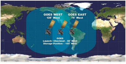
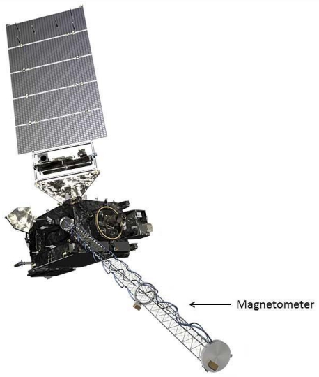
For thousands of years humans have reported paranormal phenomena such as seeing or hearing ghosts, being touched by an invisible entity, anomalous smells, etc. Because these perceived manifestations are seen, heard or felt, a physical environmental change should have occurred. While examining environmental data surrounding these perceived manifestations, a correlation between manifestations and GOES (Geostationary Operational Environmental Satellite) system magnetometer data was observed. The GOES system supports weather forecasting, severe storm tracking, and meteorology research and consists of several geosynchronous satellites and ground-based elements. The satellites are stationed above several locations around the Earth along the Equator. The one of interest in this project sits at 75 degrees W longitude at an altitude of 22,240 statute miles (GOES 13). This satellite covers East Coast, USA (figure 2 and reference 4). The magnetometer data was obtained from data compiled by NOAA from magnetometers on the satellite (figure 3). These magnetometers’ purpose is to monitor the Earth’s geomagnetic field and its variations (reference 3).
It was observed that when the magnetometer intensity readings (in nano Tesla or nT) were increasing over time, few manifestations were reported. When the magnetometer intensity readings were decreasing, however, many more manifestations were reported. During subsequent data collection excursions, this correlation seemed to exist throughout. A project was then launched to compare reports of perceived manifestations to the corresponding point on the GOES East Coast magnetometer data where the slope of the tangent line to the curve at the point in question was calculated.
Methods
Multiple excursions over time were made to locations where perceived paranormal manifestations (visual and audible) were reported along the East Coast, USA over a period of three years. Any perceived manifestations during the excursions were noted as to type, date and time. GOES magnetometer data for the East Coast (GOES 13) was then obtained from the GOES Data Access website (reference 2) for comparison. The times of perceived manifestations were then converted to UTC time to match the time zone of the GOES magnetometer readings. The slope of the tangent line for points of interest on the magnetometer data curve was then calculated and examined for magnetic field (nT) increase or decrease over time. The Microsoft Excel Slope Function was used for this calculation. Forty perceived manifestation times and forty points on the curve around the time of interest for each manifestation were used in the slope calculation. Time periods when manifestations did not occur were not included in this experiment.
Results
Data in Table 1 is only for detected manifestations. Time periods where manifestations were not detected are not included. Magnetometer data collected is in nano Tesla (nT) and is the average total magnetic field reading from all three axes of the instrument (table 2). Negative slope values indicate downward trends in the curve. Positive slope values indicate upward trends in the curve
Discussion
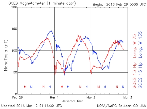
The curve created using GOES magnetometer data mimics a Sin wave in appearance with magnetic field intensity (nT) increasing and then decreasing over time. However, while the curve seems to be regular and predictable for the most part, as in any Sin wave, there are times when magnitude and frequency can change drastically very quickly (figure 1). These aberrations are not predictable, but seem to affect the reports of manifestations. The general predictability of the Sin function, though, may indicate a reason that many reports of manifestations happen at specific times at night or in the very early morning hours, especially if no curve aberration occurs.
During times when audible or visible manifestations were perceived, calculated slopes on the corresponding GOES magnetometer data indicated a mostly downward trend in intensity. During each date when manifestations were perceived, there was much time when nothing at all was perceived. For example, on 7/18/15 we were on location from 6pm until 4am the next morning with only 6 instances of perceived manifestations. This seems to show that perceived manifestations are more likely to occur when the calculated slopes indicate a downward trend in magnetic field intensity, though they could still occur less frequently when the calculated slope indicates an opposite trend. This seems to hold true during times of abnormal dips and spikes in the curve.
Anecdotal evidence also seems to indicate that manifestations may be of a more intense nature if the slope when magnetic field intensity is decreasing is more negative. However, more work needs to be performed regarding the intensity to increased negative slope correlation. More work also needs to be performed regarding perceived manifestations at locations other than East Coast, USA to see if the correlations still exist elsewhere using different GOES locations and to the time of day of reported manifestations. Finally, more work needs to be performed to compare results to magnetometer data outside the Earth’s magnetosphere to determine whether the effect is solar or terrestrial in nature.
Sources of error in this experiment could be associated with improvements in data collection over the time period reviewed and the time format for when the perception of manifestations occurred (hh:mm). For future work, the time format for data collection should be as precise as possible (hh:mm:ss.x) to match the time format used in the GOES data and data collection techniques should be consistent during the entire data collection period.
References
- http://www.swpc.noaa.gov/products/goes-magnetometer
- http://www.ngdc.noaa.gov/stp/satellite/goes/dataaccess.html
- http://www.goes-r.gov/spacesegment/mag.html
- http://www.nasa.gov/feature/goddard/nasa-celebrates-contributions-to-40-years-of-noaagoes-satellites
Figures
Tables
Table 1 – Slope Calculations
Date __ Time __ Time Zone __ UTC Date __ UTC Time __ Type __ Slope
3/1/2014 __ 8:51pm __ EST __ 3/2/2014 __ 1:51am __ A __ -122.68
3/2/2014 __ 2:51am __ EST __ 3/2/2014 __ 7:51am __ A __ 243.4745
3/2/2014 __ 4:06am __ EST __ 3/2/2014 __ 9:06am __ A __ 321.5146
6/21/2014 __ 8:05pm __ EDT __ 6/22/2014 __ 12:05am __ A __ -397.987
6/21/2014 __ 10:57pm __ EDT __ 6/22/2014 __ 2:57am __ V __ 261.2105
6/22/2014 __ 1:03am __ EDT __ 6/22/2014 __ 5:03am __ A __ -131.397
6/22/2014 __ 2:05am __ EDT __ 6/22/2014 __ 7:03am __ A __ 55.40351
7/19/2014 __ 7:44pm __ EDT __ 7/19/2014 __ 11:44pm __ A __ -192.338
7/19/2014 __ 9:58pm __ EDT __ 7/20/2014 __ 1:58am __ A __ -466.047
7/20/2014 __ 2:10am __ EDT __ 7/20/2014 __ 6:10am __ A __ 109.2283
7/20/2014 __ 3:04am __ EDT __ 7/20/2014 __ 7:04am __ A __ -66.34
9/20/2014 __ 6:18pm __ EDT __ 9/20/2014 __ 10:18pm __ A __ -179.668
9/20/2014 __ 6:47pm __ EDT __ 9/20/2014 __ 10:47pm __ A __ -875.086
9/20/2014 __ 7:08pm __ EDT __ 9/20/2014 __ 11:08pm __ A __ -180.306
10/18/2014 __ 8:51pm __ EDT __ 10/19/2014 __ 12:51am __ A __ -576.705
10/18/2014 __ 10:46pm __ EDT __ 10/19/2014 __ 2:46am __ A __ -38.304
2/21/2015 __ 7:06pm __ EST __ 2/22/2015 __ 12:06am __ A __ -2270.66
2/21/2015 __ 8:33pm __ EST __ 2/22/2015 __ 1:33am __ A __ -802.924
3/21/2015 __ 9:18pm __ EST __ 3/22/2015 __ 2:18am __ A __ 90.232
3/21/2015 __ 11:33pm __ EST __ 3/22/2015 __ 4:33am __ A __ -142.777
7/18/2015 __ 9:35pm __ EDT __ 7/19/2015 __ 1:35am __ A __ -66.33
7/18/2015 __ 10:07pm __ EDT __ 7/19/2015 __ 2:07am __ A __ 147.5342
7/18/2015 __ 10:56pm __ EDT __ 7/19/2015 __ 2:56am __ A __ -173.511
7/18/2015 __ 11:07pm __ EDT __ 7/19/2015 __ 3:07am __ V __ -178.251
7/18/2015 __ 11:09pm __ EDT __ 7/19/2015 __ 3:09am __ A __ -82.4767
7/18/2015 __ 11:16pm __ EDT __ 7/19/2015 __ 3:16am __ A __ -295.545
7/18/2015 __ 11:24pm __ EDT __ 7/19/2015 __ 3:24am __ A __ -683.542
7/18/2015 __ 11:37pm __ EDT __ 7/19/2015 __ 3:37am __ A __ -81.5228
9/12/2015 __ 6:45pm __ EDT __ 9/12/2015 __ 10:45pm __ A __ -736.576
9/12/2015 __ 9:38pm __ EDT __ 9/13/2015 __ 1:38am __ A __ -534.272
9/26/2015 __ 7:28pm __ EDT __ 9/26/2015 __ 11:28pm __ A __ -1426.66
9/26/2015 __ 8:55pm __ EDT __ 9/27/2015 __ 12:55am __ A __ -408.617
9/26/2015 __ 9:55pm __ EDT __ 9/27/2015 __ 1:55am __ A __ 267.2164
9/26/2015 __ 11:27pm __ EDT __ 9/27/2015 __ 3:27am __ A __ -229.691
10/10/2015 __ 9:49pm __ EDT __ 10/11/2015 __ 1:49am __ A __ -11275.7
10/10/2015 __ 9:59pm __ EDT __ 10/11/2015 __ 1:59am __ A __ -642.874
10/24/2015 __ 5:51pm __ EDT __ 10/24/2015 __ 9:51pm __ A __ -6380.77
10/24/2015 __ 8:32pm __ EDT __ 10/25/2015 __ 12:32am __ A __ -3407.73
2/28/2016 __ 3:10am __ EST __ 2/28/2016 __ 8:10am __ A __ -93.2336
2/28/2016 __ 3:22am __ EST __ 2/28/2016 __ 8:22am __ A __ -435.963
Table 2 – Example Raw GOES 13 Magnetometer Data (time_tag = date/time, HT_2=nT)
time_tag __ HT_2
00:00.2 __ 88.06
00:00.7 __ 88.06
00:01.2 __ 88.05
00:01.7 __ 88.06
00:02.3 __ 88.07
00:02.8 __ 88.05
00:03.3 __ 88.04
00:03.8 __ 88.02
00:04.3 __ 88.01
00:04.8 __ 88.02
00:05.3 __ 88.02
00:05.8 __ 88.02
00:06.4 __ 88.02
00:06.9 __ 88.02
00:07.4 __ 88.01
00:07.9 __ 88
00:08.4 __ 88
00:08.9 __ 88
00:09.4 __ 87.99
00:09.9 __ 87.99
00:10.4 __ 87.98
00:11.0 __ 87.98
00:11.5 __ 88
00:12.0 __ 88
00:12.5 __ 87.98
00:13.0 __ 87.97
00:13.5 __ 87.97
00:14.0 __ 87.96
00:14.5 __ 87.97
00:15.1 __ 87.96
00:15.6 __ 87.97
00:16.1 __ 87.95
00:16.6 __ 87.95
00:17.1 __ 87.94